Use cases

This section showcases example use cases of the plugin.

Mapping Cameroon forest types with Sentinel 2 data

The goal in this example is to map different forest types using multispectral Sentinel 2 data.

We have a raster and points labelled by photo-interpretation:

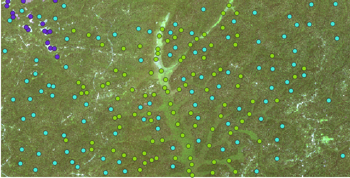
One this image, the dark blue points correspond to open forests, green to swap forests and light blue to dense forests. This dataset was randomly split into 80-20% between a train and a test set to learn a RF classifier. The image was either fed into a deep learning (DL) backbone (ViT base DINO) or not.

Here is a recap of the random forest accuracy given different pre- and post-processing of the encoder’s features.

Using a DL encoder	Pre-processing	Post-processing	Accuracy
No	No	No	0.88
Yes	No	No	0.75
No	3D PCA	No	0.93
Yes	3D PCA	No	0.86
Yes	No	10D PCA	0.86
Yes	3D PCA	10D PCA	0.90

As we can see, the use of a ViT encoder does not necessarly improve the accuracy of the calssification. Indeed, the backbone used here was trained on RGB images, working on multispectral data seems to be to far a step here. Moreover, the different forest types have allready diffrente spectral responses.

By desing, ViT are better than other ML methods to interpret the structure of an image and the relation between patches. Here, the information being mosty spectral leads to poorer performances after the use of a DL encoder, since the spectral information is drowned between unrelevant structural and tetural information interpreted by the DL backbone.

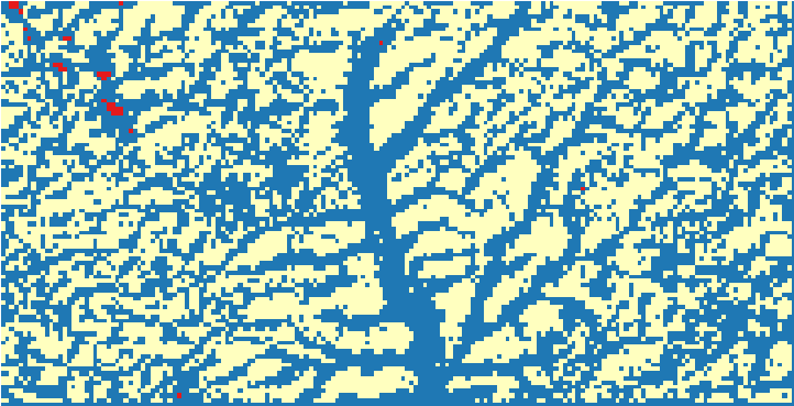
Here is the resulting map obtained when infering the RF model without pre-processing:

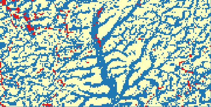
And with pre-processing:

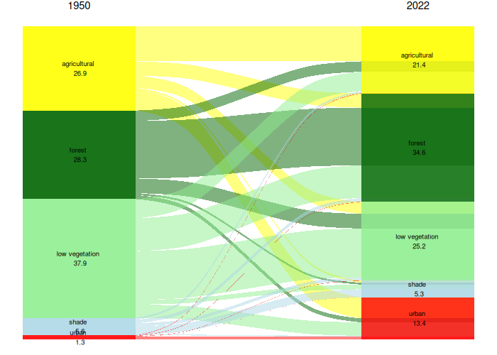
Mapping Land Cover change in La Reunion island

The objective is to characterize land cover change in La Reunion island based on the analysis of aerial IGN ortho-photography from 1950 and 2022.

Data

The data used here comprises two datasets, one of historical orthophotos from 1950 and the other of recent orthophotos from 2022.

Date	Tiles	Modality	Resolution	Source
1950	130	Grayscale (uint8)	50cm/pixel	IGN
2022	130	RGB (uint8)	20cm/pixel	IGN

Pre-processing

The recent images resolution is transformed from 20cm/pixel to 50cm/pixel using QGIS in order to obtain the same resolution as the historical images. In addition, a conversion from color (RGB or 3-bands) to grayscale (1-band) is applied using QGIS plugin OTB (OTB  > feature extraction > radiometric indices >set band 3 2 1, choosing Brightness index. Thanks to these two steps the comparison between both maps can be done pixel by pixel.

Land Cover classes :

A photo-identification is achieved on 30 randomly selected tiles for each dataset. The variability inherent to each class is accounted for by the identification of 10 polygons per landcover class for the training set and another 10 polygons per landcover class for the validation step. Training and validation sets are spatially separated to avoid spatial auto-correlation.

The different landcover classes are the following :

• Agricultural

• Low vegetation

• Forest

• Shade

• Urban

Processing

Preliminary test have been done to diffferenciate a variety of homogeneous patchs (such as forest, urban area, low vegetation) using the Haralick Texture metrics (i.e. 9 metrics from the R package GLCMTextures) with different sets of parameters and using the resulting features to train a RF classifier but the results were not satisfying, motivating the use of a DL encoder.

Images are fed through a ViT base DINO encoder with default parameters and the resulting features are used as input for a random forest classifier (ntree=500, mtry=28). The RF achieves the following kappa: 0.851 for 1950 and 0.917 for 2022

Results

Here are the classification results for 1950:

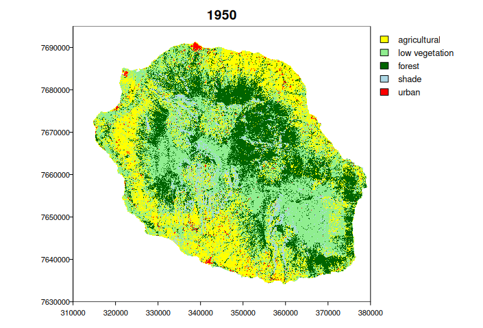
And the classification for 2022:

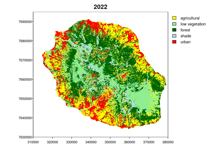
Then, we can analyze land cover changes between 1950 and 2022: